In the last post I showed how to use purrr to perform a simple Monte Carlo simulation.
Since simulation studies are usually computationally expensive, it is benifical to
write efficient code and make use of parallelization. The latter even more important when working on a modern computer.
My PC has a Ryzen 3700X CPU with 8 cores and 16 threads. For longer computations it would be a waste of
ressources not to go parallel when possible. If there is code using purrr::map_*() it is extremly simple to do so by replacing it with furrr::future_map_*().
I will use an example from econometrics where we will compare heteroscedasticity robust with non-robust standard errors when testing the hypothesis \(H_0: \beta_i = 0\) in the simple linear regression model
\[y_i = \beta_1 + \beta_2 x_i + u_i\]
where \(u_i \sim N(0, \sigma_i^2)\).
Similar to the last post I start by writing a function which…
- …generates some data (according to the simple linear regression model with either homoscedastic or heteroscedastic errors).
- …does some statistical computations (here fitting a linear model with OLS, computing standard errors, t-statistics and p-values).
- …returns a data frame with the results and the used parameters.
library(tidyverse) # contains purrr and some other packages I will use
library(furrr)

sample_t_stat <- function(n = 100, beta = c(0.5, 0.5), beta_0 = c(0, 0), error_dist = "homoscedastic",
                          standard_error = "normal"){

  # generate data
  X       <- cbind(rep(1,n), runif(n,-4,4))


  u <- switch(error_dist,
              homoscedastic     = rnorm(n, sd = 2),
              heteroscedastic   = rnorm(n, sd = sqrt(abs(X[ ,2]))), # same uncoditional variance as for homoscedasticity
              stop("Unknown distribution")
  )
  y       <- X %*% matrix(beta) + u

  # fit the model with OLS
  lin_reg <- lm.fit(X,y)

  # compute standard errors
  se <- switch(standard_error,
               normal = sqrt( (1/(n-2)*sum((lin_reg$residuals)^2) * solve(t(X) %*% X)[diag(T,2,2)])) ,
               robust = sqrt( (solve(t(X) %*% X) %*% t(X) %*% diag((lin_reg$residuals)^2) %*% X %*% solve(t(X) %*% X))[diag(T,2,2)]),
               stop("Unknown distribution")
               )

  # compute t-statistic and p-values
  t_stat  <- (lin_reg$coefficients - beta_0) / se
  p_value <- 2 * (1 - pt(abs(t_stat), df = n - 2))


  data.frame(t_stat_beta1 = t_stat[1], t_stat_beta2 = t_stat[2],
             p_value_beta1 = p_value[1], p_value_beta2 = p_value[2],
             beta1 = beta[1], beta2 = beta[2],
             beta1_0 = beta_0[1],  beta2_0 = beta_0[2],
             n, error_dist, standard_error,
             stringsAsFactors = FALSE)
}
We will look how the test performs with different sample sizes, error variances, standard errors and values for \(\beta_2\), keeping the rest of the possible input values fixed at their default values.
# considered parameter combinations
parameter_grid <- expand.grid(
  n = c(10, 50, seq(100, 500, 100)),
  beta2 = seq(-0.5,0.5, 0.1),
  error_dist = c("homoscedastic", "heteroscedastic"),
  standard_error = c("normal", "robust"),
  stringsAsFactors = FALSE
  )
The simulation for a given set of parameters is performed by mc_t_stat() which runs sim_t_stat() 1000 times.
mc_t_stat <- function(n, beta2, error_dist, standard_error){
  map_df(1:1000, ~ sample_t_stat(n = n,
                           beta = c(0.5, beta2),
                           error_dist = error_dist,
                           standard_error = standard_error)
      )
}
With the function purrr::pmap_dfr() we can iterate over the rows of the parameter grid and run mc_t_stat() for each set of parameters.
system.time(
res <- pmap_dfr(parameter_grid, mc_t_stat)
)
## user system elapsed
## 391.59 25.03 435.35This takes a while. However, if I simply add the line plan(multiprocess) and switch from
purrr::pmap_dfr() to furrr::future_pmap_dfr() the computation time on my computer is reduced significantly.
library(furrr)
plan(multiprocess)
system.time(
res2 <- future_pmap_dfr(parameter_grid, mc_t_stat)
)
## user system elapsed
## 0.28 0.03 39.69I think this is one of the easiest ways to parallelization in R. The future.apply package does the same for the apply functions, in case you like those more.
Finally, a quick look at the results.
res2 %>%
  group_by(n, error_dist, standard_error , beta2) %>%
  summarise(rejection_rate = mean(p_value_beta2 < 0.05)) %>%
  ggplot(aes(x = beta2, y = rejection_rate, col = standard_error )) +
  facet_grid(n ~ error_dist) +
  geom_line() +
  geom_abline(intercept = 0.05, slope = 0, linetype = "dashed")  +
  geom_vline(aes(xintercept = 0), linetype = "dashed")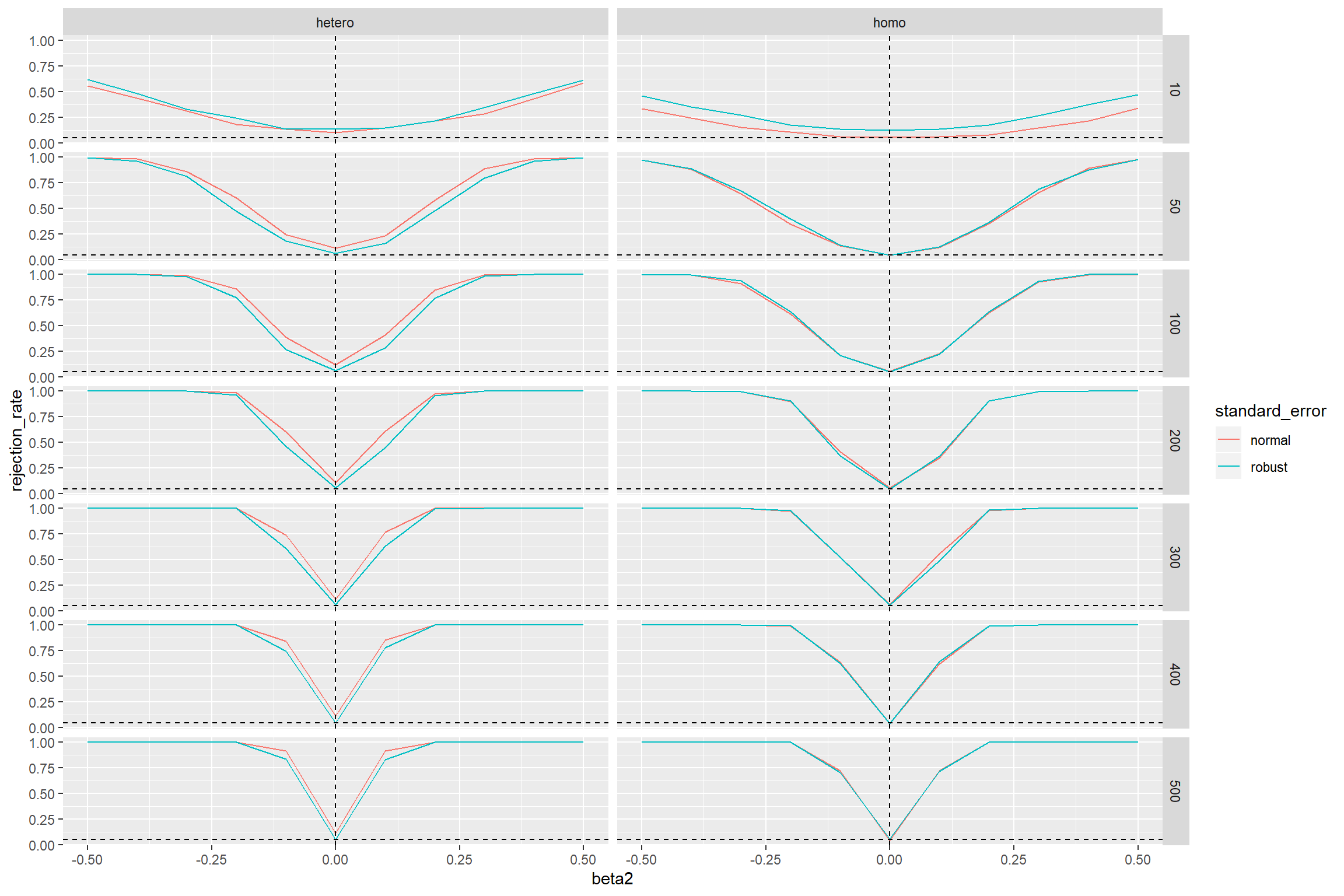
We would expect that the test rejects in 5 percent of the cases if the null hypothesis is true. That is the case when \(\beta_2 = 0\). However, we find that under heteroscedasticity the test with the non-robust standard errors rejects too often (the curves should go through the point where the two dashed lines intersect). This doesn’t even change when the sample size increases. The test with robust standard errors is doing here a much better job.
If the errors are homoscedastic, both tests perform for sample sizes of approx. 100 and more almost equally well.